Overview of Statistical Techniques


Below, I give an overview of new statistical methods that are introduced in Science: Under Submission and provide links to the relevant Matlab code. I do not reflect on the foundations of science and statistics here, but just summarize the techniques that are proposed in the book.

To introduce some notation, say a detective wants to estimate a person's height (in cm) on the basis of her (or his) length of the right foot (in cm). The following formula could be used to estimate the height of a person,

estimated height = 17 + 6 × length right foot.

The bigger the right foot is, the taller a person is estimated to be. For a data set of N observations, the estimated height of person n = 1, 2, ..., N is referred to as ŷn. The values 17 and 6 are called parameters and are denoted as b0 and b1 respectively. These parameter values have been optimized on the basis of a data set. In a model such as this, the length of the right foot of a person is known as the regressor xn,1. If we allow for multiple regressors xn,k with k = 1, 2, ..., K to predict a person's height, the linear regression model is given by

ŷ n = b0 + b1xn,1 + b2xn,2 ... + bKxn,K.

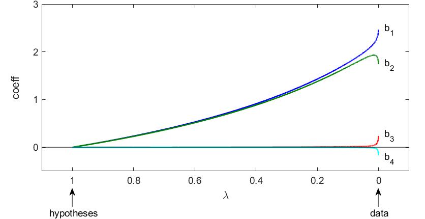
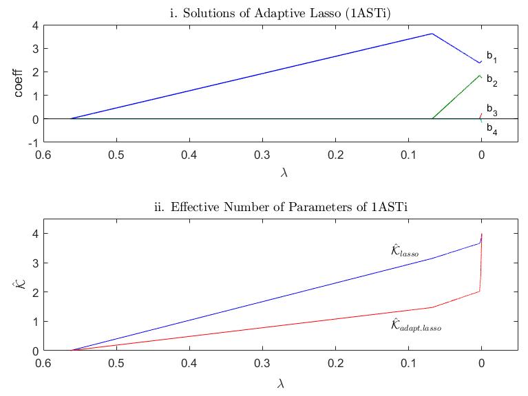
A researcher might have hypothesized that the length of a person increases by 4 rather than 6 times the length of the right foot. Current statistical techniques hardly enable a researcher to anticipate and influence how the in-sample accuracy of the data-optimized solutions is balanced with the simplicity of sticking to the hypotheses. I offer an intuitive approach to control such an accuracy-simplicity tradeoff (AST).

CH 7: b2ASTc

When estimating parameters of the linear regression model, statistical techniques often use a tuning parameter λ to determine what the relative influence of the hypothesis is compared to the data-optimized solution. A λ value may vary between 0 and infinity and it is unclear before analyzing the data what degree of shrinkage towards the hypotheses is associated with a given level of λ. I show how these techniques can be rescaled so that the interpretation of λ does become straightforward. For uncorrelated regressors, λ×100% indicates in percentage terms what the minimal influence of the hypothesis is relative to the data-optimized solution. The smaller a regressor's contribution is to the famous R2 measure of fit, the more the parameter is further shrunk towards the hypothesis. I now present a technique of mine that also enables one to deal with cross-correlations between regressors.

Figure 1: b2ASTc
b2ast

In Figure 1, a simulated data set of size 20 is used whereby the first two regressors are relevant and highly correlated while the third and fourth regressors are irrelevant and uncorrelated. The hypothesis is that all parameter values are equal to zero, but this setting may be altered. Observe that the hypothesized values are always selected when λ equals 1. The data-optimized solutions are chosen when λ equals 0. The in-sample accuracy of the hypothesized model is improved by R2 = 97% when the data-optimized solutions are used.

The regressors x1 and x2 each contribute around 48% to the total R2 accuracy of 97%. That is why their parameters are shrunk almost linearly towards the hypothesis of zero as λ increases to one. Since x1 and x2 are highly correlated, they are stimulated to receive a similar deviation from the hypothesis of zero. The user can specify how high the absolute cross-correlation needs to be for parameters to be 'grouped' in this way. Here, I have set this tuning parameter to 0.5. The third and fourth regressors are barely correlated with other regressors, so grouping is not promoted for their parameters. Since they also barely contribute to R2 accuracy, b3 and b4 are already nearly equal to zero for tiny λ values.

The above illustrated method is referred to as b2ASTc. The 2 in the subscript signifies that a model's simplicity is measured by taking squared deviations from the hypotheses. The 'c' indicates that cross-correlations are accounted for. Aside from introducing b2ASTc, I give a formula for decomposing R2, present an AST-scaled version of ridge (and Bayesian) regression, and indicate how estimators with an AST are related to Zellner's g-prior.


CH 8: b1ASTc

Estimators that use absolute values rather than squared values to measure a model's simplicity have a property that is convenient for the interpretation of the solutions. They perform exact subset selection, which means that parameters are exactly equated to the hypothesized parameter value before λ has reached its maximum. So far, we have not been able to interpret the λ value at which a parameter is allowed to deviate from the hypothesized parameters. I show that such moments of activation are directly related to a regressor's contribution to R2 accuracy, also when the hypotheses deviate from zero. This interpretation of λ enables us to anticipate and influence the effect of hypotheses on parameter estimates. The technique I introduce is called b1ASTc. The '1' in the subscript indicates that absolute deviations from the hypotheses are computed to measure the simplicity of a model. The 'c' means that the influence of correlations on the grouping of parameters is controlled as well.

Figure 2: b1ASTc and Diabetes
b1ast

Figure 2 gives an illustration whereby a case study is used with 442 diabetes patients (Efron, 2004). A measure of how diabetes progressed one year after a baseline is regressed on ten baseline variables. The explanatory variables are age, sex, body mass index (BMI), average blood pressure (BP) and six blood serum measurements. The hypothesis is that all of these regressors are irrelevant, which implies that the regression coefficients are conjectured to be zero. The in-sample accuracy of the hypothesized model is improved by an R2 of 52% when the data-optimized solutions at λ = 0 are used. After compensating for high cross-correlations, the fifth blood serum and the body mass index are activated at λ values of around 0.20, as Figure 2 shows. This means that they each contribute around 20% to R2 accuracy and account for the lion's share of the model's in-sample fit. Such interpretations about λ were not available before. The researcher can again specify how high cross-correlations need to be for parameters to be grouped together. AST-scaled versions of the popular lasso, adaptive lasso, and the elastic net are also provided, so that their behavior becomes easy to control through λ as well.

CH 9: AST and the Selection of Tuning Parameters

Although estimators with an AST make it easy to anticipate and influence how the tuning parameter λ balances between hypotheses and data-optimized solutions, researchers might still want to make the choice of λ dependent on the data. Cross-validation and information criteria are well known techniques for choosing a model. I show how a practitioner can intuitively balance between her own estimate of λ and the cross-validated alternative by formulating another AST. Information criteria are heuristics that select a model by optimizing over its in-sample accuracy while minimizing over its effective number of parameters. Currently, the two main available methods for measuring the effective number of parameters have both become controversial. I show that this controversy is based on a false premise and offer a straightforward way of counting the number of parameters.

If only one out of two regression parameters is allowed to deviate from zero, the intuition might be that the estimated number of parameters in that sub-model should not exceed 2 — but that intuition is wrong. A model with fewer regressors may need to be penalized harder by increasing the effective number of parameters in order to avoid relevant regressors with high cross-correlations from being arbitrarily excluded. The literature has not recognized this important issue. In predicting a person's height, for instance, the F-test arbitrarily ignores the left foot if the right foot is already included in the model, because it does not compensate for high cross-correlations in counting the number of parameters. This problem can easily be solved. Estimators with an AST use a simplicity term to measure deviations from a hypothesis and I argue that an estimator's simplicity term can directly be used as its measure for the effective number of parameters.

Figure 3
Khat

The upper panel of Figure 3 shows how an AST-scaled version of the adaptive lasso shrinks parameters to zero when the first two regressors are simulated to be equally relevant and highly correlated and the third and fourth regressors are simulated to be irrelevant and uncorrelated. Observe that for many values of λ, the estimator arbitrarily singles out the first regressor while ignoring the almost equally relevant and highly correlated second regressor.

    The lower panel indicates how the simplicity terms of the lasso and the adaptive lasso count the effective number of parameters of the candidate models in the upper panel. To penalize the arbitrary exclusion of the second regressor, the effective number of parameters exceeds 2 for the lasso even before the second parameter is added to the model at λ = 0.07. Observe also that the lasso gives a higher penalty for ignoring correlated regressors than the adaptive lasso. This corresponds to the finding in Chapter 8 that the lasso promotes grouping more strongly than the adaptive lasso. Reasons for preferring one measure of the effective number of parameters over another are thus largely the same as those for preferring one estimator over another.

  • Download book (Ch 9)
  • Download code (Ch 7-9)

CH 12: AST and Weighing Observations

The forecasting performance of a model can change over time. To deal with such changes, one can estimate the optimal timing of the starting point of a data set and use post-break data. This is called the best starting point method (SPB). I make three ad hoc improvements by analyzing SPB's performance in simulation studies and empirical applications. First, the response time to a new break can be shortened by weighing observations exponentially after a recent break. Second, it can be remarked that observations before a break need not be ignored altogether, because these observations can be of relevance in the future. This is another accuracy-simplicity tradeoff between the accuracy of recent prediction errors and the simplicity of sticking to equal weights. Third, individual weights could be assigned to multiple periods instead of only using post-break observations.

Figure 4
Weigh

Figure 4 shows how the proposed method assigns weights to the data when the objective is to predict the next observation of y by taking a weighted average of previous observations of y. In the simulated data set, the level of y increases from around 3 to 5 at T = 51 and returns to 3 at T = 90. Equal weights are used before the first break at T = 51 and exponential weights are used afterwards. In the second period at T: [51, 89], observations of the first period are not ignored completely and this reduces the prediction error at T = 90 when y jumps back to 3. The algorithm enables individual periods to receive individual weights. Accordingly, at T = 120, the first period is more emphasized than the second period.

CH 13: A Quick Search for Finding Optimal Configurations

Statistical configurations like the choice of the tuning parameter λ or the starting point of a data set are often selected on the basis of data. The general procedure is to evaluate the performance of many candidate configurations and to select the best one. If some configuration is defined between -1 and +1, the strategy of the grid search is to equally spread candidate configurations over the space, so c = -1, -0.99, -0.98, ..., 0.98, 0.99, 1. If two sets of forecasts are (nearly) the same for c = -1 and c = -0.75, then it might be a waste of time to consider configurations that lie in between. So, one approach towards expanding the configuration set is to find out where the average forecasting deviance (FD) between two consecutive configurations is largest and add the point that lies in the middle. Another approach is to add a candidate c that lies between two consecutive configurations which have on average the best forecasting accuracy (FA) according to some loss function. The FAD (forecasting, accuracy, deviance) approach gives the user control over the gradual transition from an FD to an FA search, so that multiple minima can be identified.

Figure 5
Search

Figure 5 shows how the FAD search adds candidate configuration for each new run in case there are two minima (red dotted lines). For the purpose of illustration, I indicate what happens if the user specifies that 200 candidate configurations are to be considered rather than, say, 10. Instead of adding more configurations redundantly close to the best configuration observed so far, FAD will keep on looking for alternative local minima in a systematic fashion. I compare FAD's performance with the grid, random, and expected improvement search techniques in terms of accuracy and computational speed for when there are single and multiple statistical decisions that are optimized over. The FAD procedure shows promising results and particularly if configurations that are closer together generally have more similar forecasts.